Comparing supervised machine learning algorithms in classifying wine quality
This paper was originally written as a final project for PSTAT 131 Data Mining at UC Santa Barbara in spring 2017. It was revised heavily for STATS 295 Advanced R at UC Irvine. A version of this project written in Python can be found on my GitHub here.
Abstract
There are many different machine learning techniques useful for classification. This paper compares various supervised learning algorithms, namely decision trees, k-nearest neighbors, and random forest in order to determine which is the most effective for binary classification. The usefulness of cross-validation and the necessity of randomness to ensure robustness is also discussed in this paper. We utilize a free and openly sourced dataset available on the UC Irvine Machine Learning Repository which includes several different attributes of wine including alcohol content, sulfur dioxide, and acidity, among others, and use these different ML algorithms to classify each of them as either good or bad. We found that the models that performed the best overall were random forest, but acknowledge that they suffer from a lack of interpretability on account of being a black-box algorithm.
Introduction
The importance of identifying what constitutes wine quality is a question of interest to many; whether you produce wine or consume it. While wine tasting as a profession has a long history, the application of statistics and machine learning to determine wine quality is comparatively much younger. Taking a dataset that has pre-existing quality scores assigned to different wines, we can apply supervised learning machine learning algorithms to attempt to determine which among them performs best when classifying the quality of the wine, and what attributes they determined were the most relevant in that classification.
Background
We use this white wine quality dataset, and all of its attributes (e.g. sulfur dioxide content, pH) to determine what constitutes a “good” (or above average) quality wine. We used the R statistical computing language to conduct the analyses in this report. The data were found on the UC Irvine Machine Learning Repository (“UCI Machine Learning Repository” n.d.).
Knowing what makes a good wine was an interesting question because it allows us to look at “taste” in a different way–without formal training in wine tasting, we can determine algorithmically how and why a wine is good using machine learning.
We utilized random forest, decision trees, and k-nearest neighbors to classify each observation as either good or bad based off of these attributes, while varying the number of variables, nodes, and number of neighbors and comparing within and between these methods.
In this report, we find the accuracy, error rates, and area under the ROC curve (AUC) of each of the three methods and ultimately came to determine that random forest was the most effective in terms of accuracy and AUC. It works well as a generalization of the decision tree method, and as an algorithm it is robust, but it falls short in terms of interpretability. kNN on the other hand is slow to compute with a dataset of this dimensionality, as well as weaker in its accuracy both in absolute terms and relative to the other methods we have tested here.
Methods
First we can look at the correlation matrix of the dataset, to see if any predictors are highly correlated with one another. We may have to take out these predictors in order to avoid multicollinearity, which can invalidate results. Having said this, multicollinearity is less of an issue with decision trees, and even less so with random forest, both of which are going to be used in this analysis. See Figure @ref(fig:correlation-matrix) for the correlation matrix.
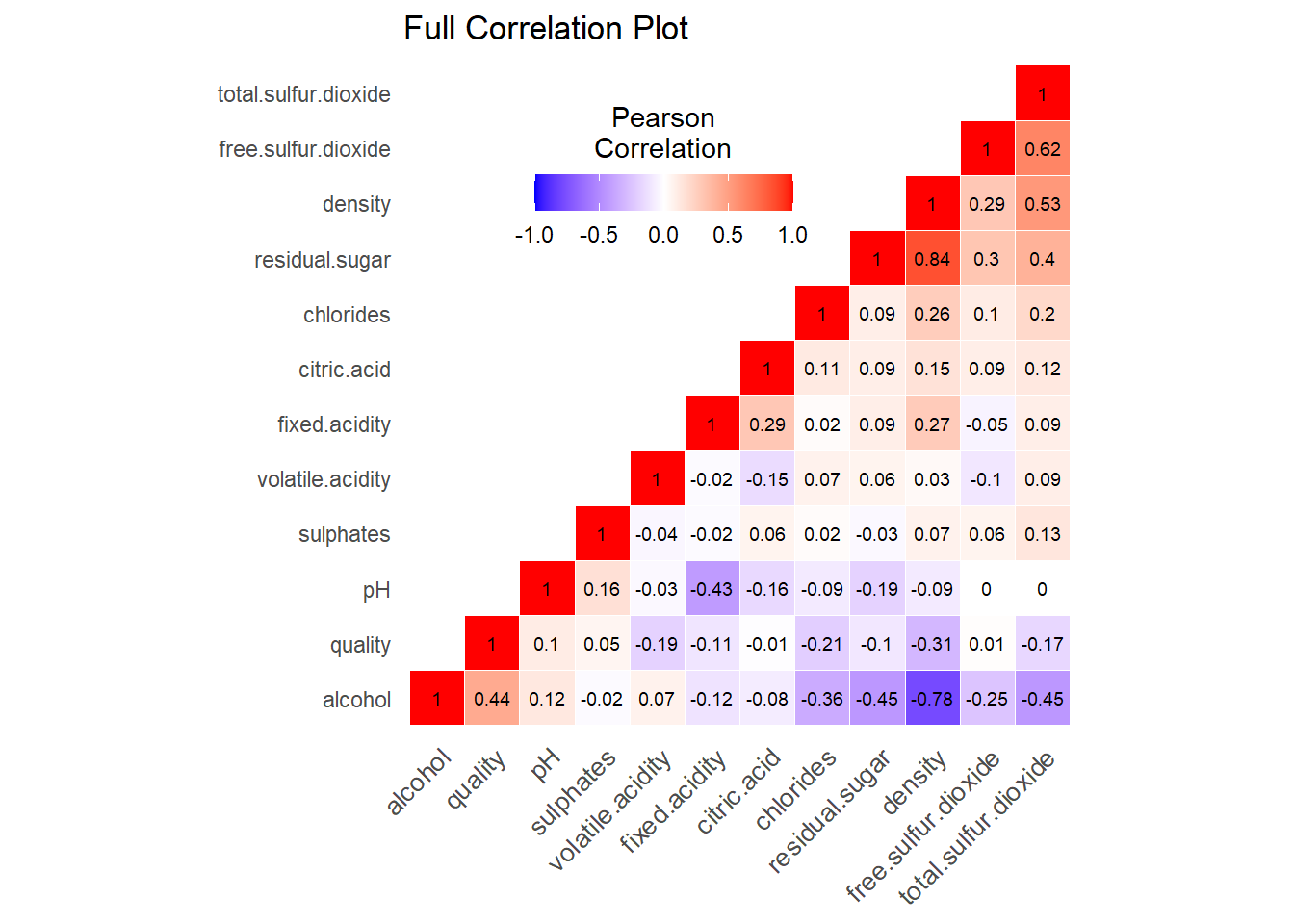
The full correlation matrix of the data.
Taking a look at the correlation coefficients \(r\) for the predictor variables, we see
that density is strongly correlated with
residual.sugar (\(r =
0.84\)) and alcohol (\(r =
-0.78\)), and moderately correlated with
total.sulfur.dioxide (\(r =
0.53\)). free.sulfur.dioxide and
total.sulfur.dioxide are also moderately correlated with
each other (\(r = 0.62\)) although this
is trivially known because of course, free sulfur dioxide is
incorporated into the total sulfur dioxide.
Aside from that correlations are all very low, including (and
especially) quality, the response variable, with the
predictors.
So, we should actually remove the variables
residual.sugar and density, as well as
total.sulfur.dioxide because if its direct relationship
with free.sulfur.dioxide, in order to address problems with
multi-collinearity. We’re going to withhold removing
alcohol, to see the if the initial effect of removing just
these three correlated variables is enough to address the issue. Then
we’ll show a new correlation matrix. See Figure
@ref(fig:correlation-matrix2).
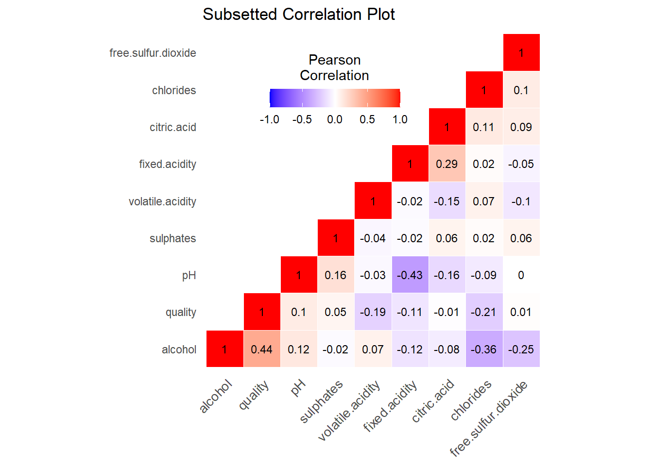
The correlation matrix without residual sugar, density, or total sulfur dioxide.
From the new correlation matrix it appears that none of the predictors now have too high or a correlation with each other, and we can decide that multi-collinearity is no longer an issue.
From here on out, we’re also going to want to convert the
quality response variable into a binary factor so that we
can use the predictors to classify the observations. We’re going to do
this by labeling all of the observations that have received an above
average (5 out of 10) as “good”, and the rest as “bad”, “bad” really
meaning “not good”.
It’s important to note that all of these numeric predictor variables
(fixed.acidity, volatile.acidity,
citric.acid, chlorides,
free.sulfur.dioxide, pH,
sulphates, alcohol) are not all scaled the
same. As such, it’s appropriate to scale them before running any further
analyses.
# to circumvent the issue of scale() changing to a matrix
scale_this <- function(x) as.vector(scale(x))

# scaling the 8 numeric attributes
white_sc <- white2 %>%
  mutate_at(vars(-quality), .funs = scale_this
  )

# Converting quality into a binary factor
white_sc <- white_sc %>%
  mutate_at(vars(quality), ~ ifelse(quality > 5, yes = "good",
                                    no = "bad")) %>%
  mutate_at(vars(quality), ~ factor(quality,
                                    labels = c("bad", "good")))
Now we have 8 numeric predictor variables, and one two-level
categorical variable (quality). We’re going to apply a few
different classification methods in order to firstly determine which the
best model for predicting is in terms of the relevant variables, and
secondly to find the best classification algorithm for this data.
In order to apply machine learning algorithms to this dataset, we need to stratify the dataset into a training set and a test set. The first set will be used to teach the classification model how to predict, depending on the algorithm chosen. We then apply the algorithm to the test set, and see how accurate the classification was.
# using a subset of 1000 obs for the training set
set.seed(10)
test_indices <- sample(1:nrow(white_sc), 1000)
test <- white_sc %>% slice(test_indices)
train <- white_sc %>% slice(-test_indices)
Decision Tree
The first method we are going to perform on this dataset, is Decision
Trees. Decision tree is a non-parametric classification method, which
uses a set of rules to predict that each observation belongs to the most
commonly occurring class label of training data [tan_introduction_2019].
We’re going to build these models using the rpart package
in R (Therneau and Atkinson 2019).
Of course, we’re going to use quality as a response
variable, and each of the now 8 remaining numeric attributes as
predictors.
Repeated k-fold Cross Validation and Pruning
We can use k-fold cross-validation, which randomly partitions the dataset into folds of similar size, to see if the tree requires any pruning which can improve the model’s accuracy as well as make it more interpretable for us.
In k-fold cross validation, we divide the sample into k
sub samples, then train the model on k-1 samples, leaving
one as a holdout sample. We compute validation error on each of these
samples, then average the validation error of all of them.
The idea of cross-validation is that it will sample multiple times from the training set, with different separations. Ultimately, this creates a more robust model i.e. the tree will not be overfit.
We can further optimize and reduce overfitting by doing repeated k-fold cross validation which replicates the procedure multiple times and reports the mean performance across all folds and repeats. Overfitting refers to when a model is trained such that it can “predict” labels extremely well for the training data but very poorly for any data it hasn’t yet seen, such as a test set or even brand new data. There are two kinds of errors committed by a classification model: training errors and generalization errors (Tan et al. 2019). The former refers to misclassification on the training data while the later refers to misclassification on unseen data (such as the test data). Ideally we would like to minimize both.
Cross validation will help us find the optimal complexity value for
the tree that yields the best accuracy while also being extremely
robust. This method using the caret (Kuhn 2020) package finds the optimal complexity
parameter (“cp”) for tuning and prunes the tree
accordingly.
Generally speaking, un-pruned decision trees that do not leverage cross-validation are prone to overfitting because they lack the element of randomness and also being overly complex. By building the model by using cross-validation to optimize the complexity parameter which determines the size of the tree, while also doing repeated random samples on the training data, we can end up with a simple, yet optimized tree that is robust and less prone to overfitting. See Figure @ref(fig:decision-tree-plot) for the decision tree plot.
# library(rpart) and library(caret) are loaded
# 10-fold cross validation repeated 3 times
set.seed(10)
caret_control <- trainControl(method = "repeatedcv",
                              number = 10, repeats = 3)

# Training the rpart decision tree based on the repeated cross-validation
# library(e1071) is loaded
tree_cv <- train(quality ~ .,
  data = train,
  method = "rpart",
  trControl = caret_control
)

# storing final model
tree <- tree_cv$finalModel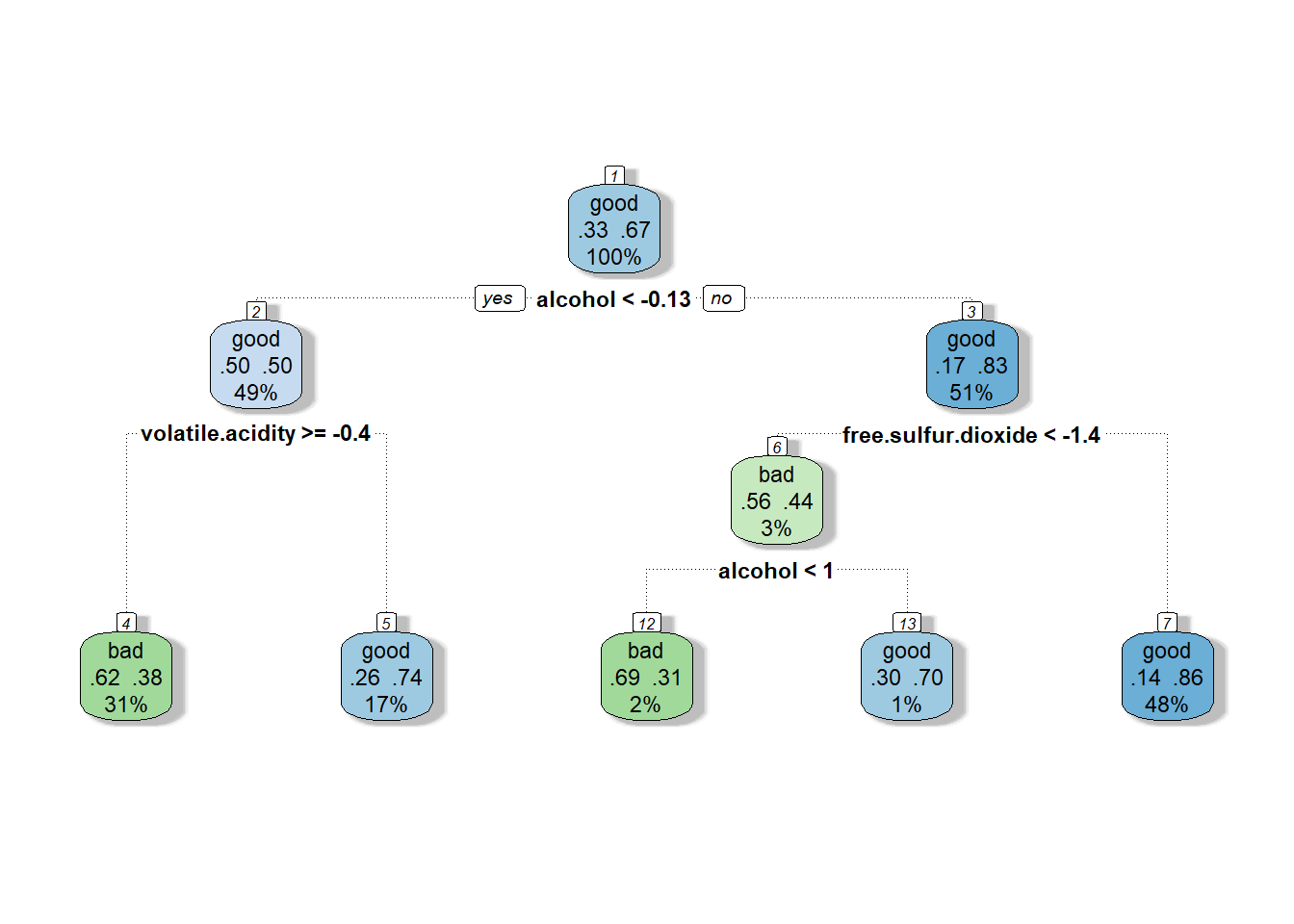
Decision tree built using rpart and 10-fold repeated cross-validation 3 times.
We can see while looking at the tree how often alcohol
appears and intuit from that that the amount of alcohol, whether high or
low, plays at least some part in the model’s classification of a good
wine. We also notice that the variables actually used in the
construction of the tree were alcohol,
free.sulfur.dioxide, and volatile.acidity.
It’s notable that this decision tree doesn’t have many “leaves” because
we used the optimal complexity parameter that came from the repeated
cross-validation step.
We can build a confusion matrix after using the data to predict on the test set, and then find the accuracy rate and the error rate. The confusion matrix is depicted as Table @ref(tab:tree-confusion-matrix).
As an alternative metric to quantify the robustness of this method,
we can use the Receiver Operating Characteristic (ROC) curve and the
area underneath it (AUC). The ROC curve plots the false positive rate
against the true positive rate, and the area underneath it falls between
either 0.5 or 1, 0.5 being the worst (random classification), and 1
being the best (perfect classification). We can build the ROC curve and
calculate the area underneath it using the ROCR package in
R (Sing et al. 2020).
The Table @ref(tab:records-1) shows the accuracy and error rate as well as AUC for the decision tree model we have built. The ROC curve itself can be seen in Figure @ref(fig:tree-ROC-curve).
# a function that returns the accuracy of a confusion matrix
class_acc <- function(conf) {
  sum(diag(conf)) / sum(conf)
}

tree_pred <- predict(tree, test, type = "class")
# confusion matrix
tree_conf <- table(pred = tree_pred, true = test$quality)

# the class_acc() function is defined locally
tree_acc <- class_acc(tree_conf)
# misclassification error
tree_err <- 1 - tree_acc

# library(ROCR is loaded)
# getting matrix of predicted class probabilities
all_tree_probs <- as.data.frame(predict(tree, test, type = "prob"))
tree_probs <- all_tree_probs[, 2]

tree_roc_pred <- prediction(tree_probs, test$quality)
tree_roc_perf <- performance(tree_roc_pred, "tpr", "fpr")

# Area under the curve
tree_auc_perf <- performance(tree_roc_pred, "auc")
tree_auc <- round(tree_auc_perf@y.values[[1]], 3)| bad | good | |
|---|---|---|
| bad | 229 | 132 |
| good | 129 | 510 |
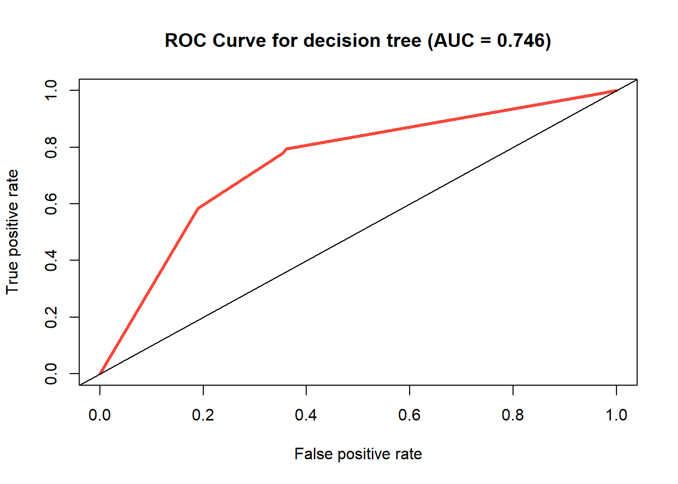
ROC curve of the decision tree model.
| Accuracy Rate | Error Rate | AUC | |
|---|---|---|---|
| Repeated Cross-Validated Decision Tree | 0.739 | 0.261 | 0.746 |
| k=10 k-Nearest Neighbors | NA | NA | NA |
| k=35 k-Nearest Neighbors | NA | NA | NA |
| full Random Forest | NA | NA | NA |
| small Random Forest | NA | NA | NA |
With an accuracy rate of 0.739, this decision tree model
is not superb, but will still classify correctly about 3 out of 4 times.
The area under the ROC curve is about 0.746, which is halfway between
randomness (0) and a perfect model (1), showing a rather mediocre model.
A perfect right angle in the upper left would indicate a perfect model
and an AUC of 1, and a diagonal (as shown in the plot) depicts an AUC of
0.5, indicating an equal chance of a false positive and a true
positive.
Having appraised this decision tree model by its accuracy rate, error rate, and AUC, we can now we can proceed to the next method of classification.
k-Nearest Neighbors (kNN)
We’re now going to apply the k-nearest neighbors method of
classification, which is a non-parametric method. k-Nearest neighbors
(or kNN) is called a “lazy learning” technique because it goes through
the training set every time it predicts a test sample’s quality (Tan et al. 2019). It finds this quality by
plotting the test sample in the same dimensional space as the training
data, then classifies it based on the “k nearest neighbor(s)”, i.e. if k
= 10, then the quality of the 10 nearest neighbors in the training data
to the test data observation will be applied to that observation. We’re
going to fit this model using the class package in R (Ripley 2020).
Distance is measured in different ways, but by default the
knn() function utilizes Euclidean distance.
This is rather problematic because when calculating distance it’s assumed that attributes have the same effect, while this is not generally true. So the distance metric (Euclidean distance in this case) does not take into account the attributes’ relationships with each other, which can result in misclassification. So already we have determined a shortcoming in the kNN method before we have even applied it. Although of course, we already dropped the predictors that were highly correlated with each other, and what’s more we scaled the remaining numeric predictors, which goes in a small way to addressing this.
We’ll build a preliminary model using k = 10, calculate the accuracy and error rates as well as the AUC, and compare them with the previous model we build using decision trees. The confusion matrix for the model is in Table @ref(tab:knn-confusion-matrix). The comparison between this model and the decision tree model can be seen in Table @ref(tab:records-2). The ROC curve itself can be seen in Figure @ref(fig:knn-roc-curve).
# library(class) is loaded
# using 10 nearest neighbors
set.seed(10)
knn_pred <- knn(
  train = train[, -9],
  test = test[, -9],
  cl = train$quality,
  k = 10,
  prob = T
)

# confusion matrix
knn_conf <- table(pred = knn_pred, true = test$quality)

# accuracy
knn_acc <- class_acc(knn_conf)
# misclassification error
knn_err <- 1 - knn_acc

# Creating the ROC curve for knn
knn_prob <- attr(knn_pred, "prob")
knn_prob <- 2 * ifelse(knn_pred == "-1", 1 - knn_prob, knn_prob) - 1
knn_roc_pred <- prediction(predictions = knn_prob, labels = test$quality)
knn_roc_perf <- performance(knn_roc_pred,
  measure = "tpr", x.measure = "fpr"
)

# Area under the knn curve
knn_auc_perf <- performance(knn_roc_pred, measure = "auc")
knn_auc <- round(knn_auc_perf@y.values[[1]], 3)| bad | good | |
|---|---|---|
| bad | 205 | 91 |
| good | 153 | 551 |
| Accuracy Rate | Error Rate | AUC | |
|---|---|---|---|
| Repeated Cross-Validated Decision Tree | 0.739 | 0.261 | 0.746 |
| k=10 k-Nearest Neighbors | 0.756 | 0.244 | 0.689 |
| k=35 k-Nearest Neighbors | NA | NA | NA |
| full Random Forest | NA | NA | NA |
| small Random Forest | NA | NA | NA |
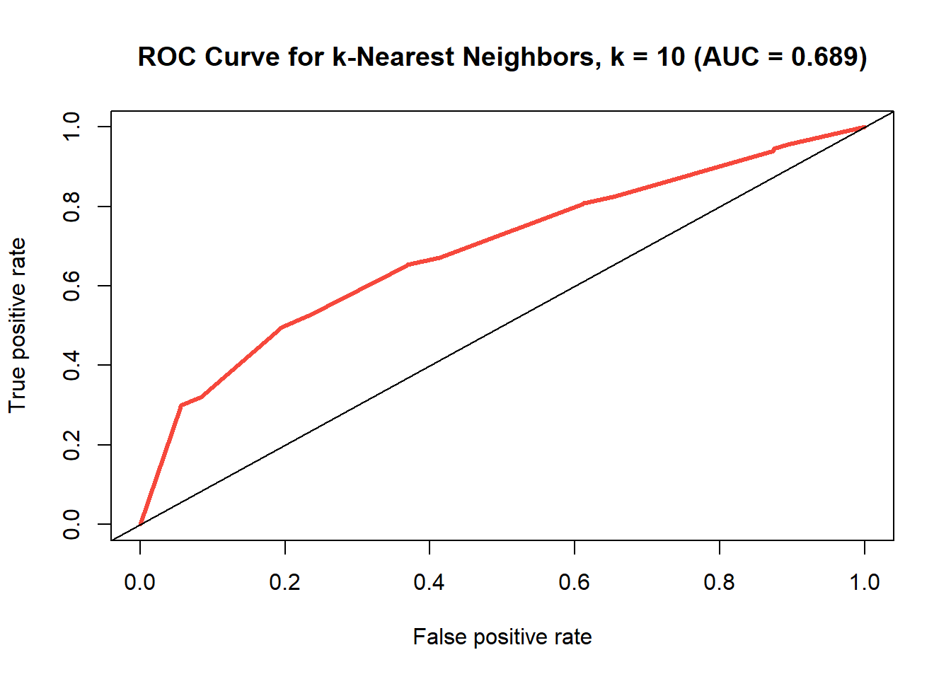
ROC curve of the k-nearest neighbors model where k=10.
So with k=10, the k-nearest neighbors model ended up with another mediocre accuracy rate (0.756). So with an AUC of 0.715, this test is not very good, but performed similarly to that of the decision tree model. We can look at different values for k and try to find the best one to use and then compare the results from that with these. Figure @ref(fig:finding-best-k) depicts this as a scatterplot of k against accuracy.
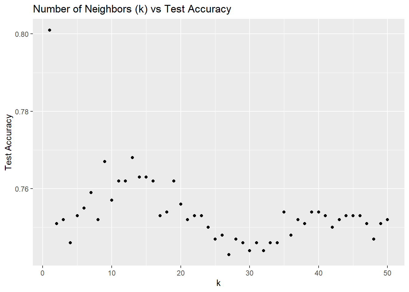
Testing various values of k with the k-nearest neighbors algorithm, and comparing accuracies.
This is interesting because accuracy seems to increase gradually, hit a peak, decrease again and slightly increase. We know well that using k = 1 will result in a very low bias and high variance, and this also means that we are fitting too closely to the training dataset and therefore, overfitting. This makes for a bad model that cannot be well generalized to new data.
Figure @ref(fig:worst-knn) demonstrates this.
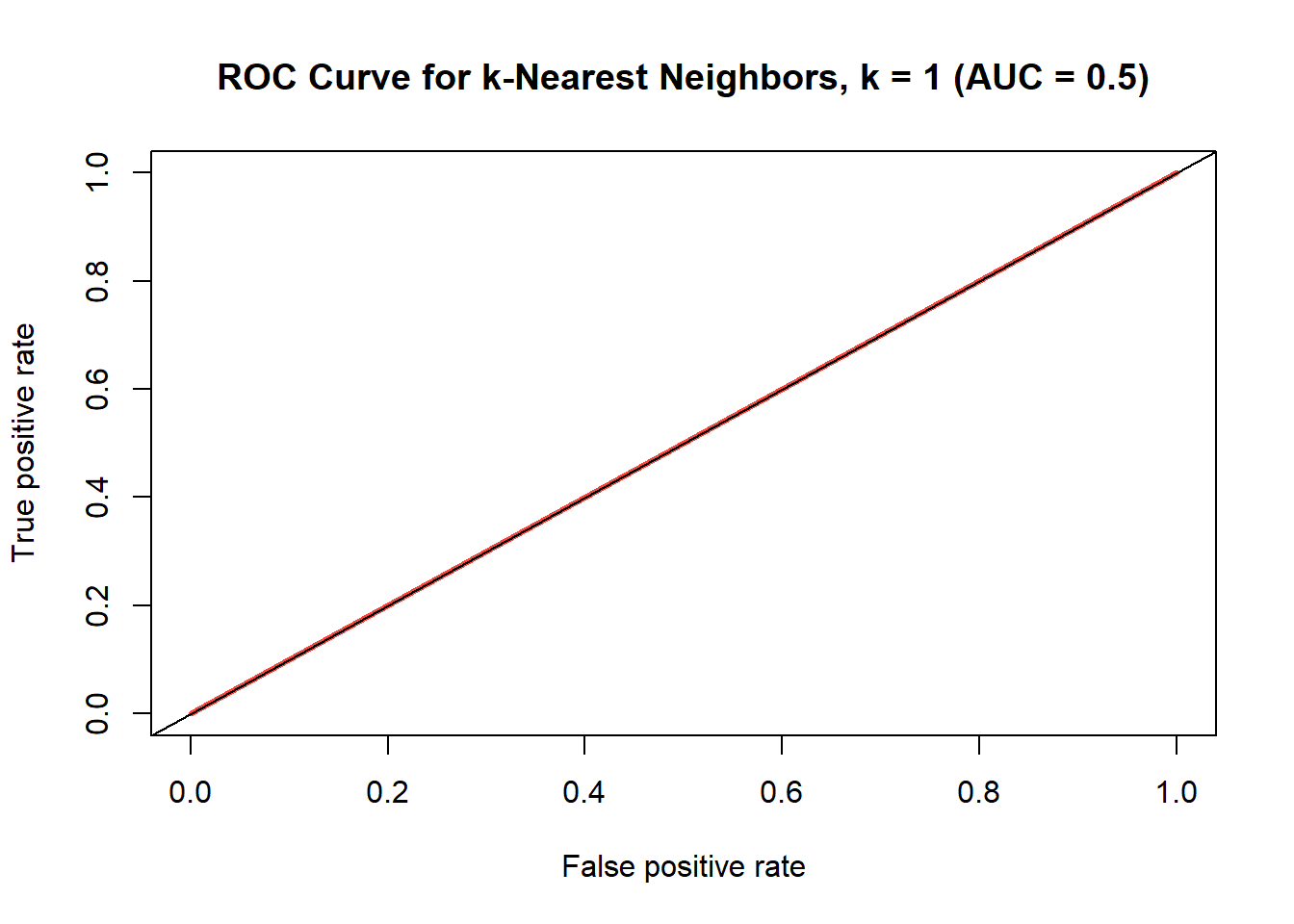
ROC curve for k-nearest neighbors model where k=1
Note that the AUC is 0.5, which is the worst possible result since it is randomly guessing (it has the same chance of a true positive as it does a false positive). So we think better not to opt for k = 1 and rather choose some k like 35, which is still decently accurate, and probably less biased. The confusion matrix for the k = 35 model can be seen in Table @ref(tab:knn-35-confusion-matrix). As with the prior models we’ll calculate the accuracy and error rate as well as the AUC, and plot the ROC curve, which can be seen in Figure @ref(fig:knn35).
The comparison of accuracy rates, error rates, and AUCs is seen in Table @ref(tab:records-2).
# library(knn) is loaded
new_knn_pred <- knn(
  train = train[, -9],
  test = test[, -9],
  cl = train$quality,
  k = 35,
  prob = T
)

# confusion matrix
new_knn_conf <- table(true = test$quality, pred = new_knn_pred)
# accuracy rate
new_knn_acc <- class_acc(new_knn_conf)
# misclassification error rate
new_knn_err <- 1 - new_knn_acc

# Creating the ROC curve for knn
# library(dplyr) is loaded
new_knn_prob <- attr(new_knn_pred, "prob")
new_knn_prob <- 2 * ifelse(new_knn_pred == "-1",
                           1 - new_knn_prob, new_knn_prob) - 1
new_knn_roc_pred <- prediction(
  predictions = new_knn_prob,
  labels = test$quality
)
new_knn_roc_perf <- performance(new_knn_roc_pred,
                                measure = "tpr",
                                x.measure = "fpr")

# Area under the knn curve
new_knn_auc_perf <- performance(new_knn_roc_pred, measure = "auc")
new_knn_auc <- round(new_knn_auc_perf@y.values[[1]], 3)| bad | good | |
|---|---|---|
| bad | 197 | 161 |
| good | 84 | 558 |
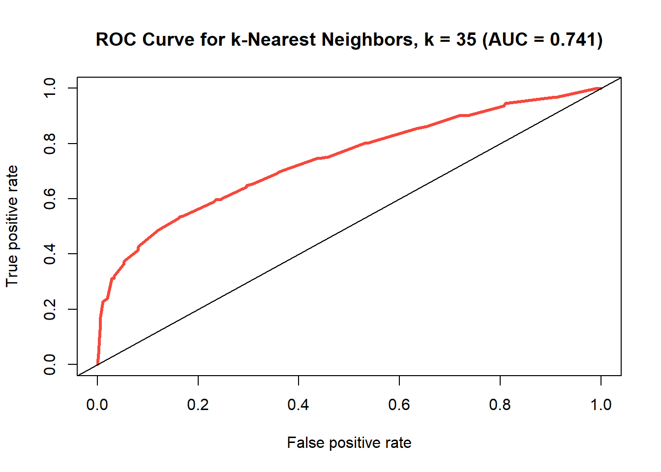
ROC curve for k-nearest neighbors model where k=35
| Accuracy Rate | Error Rate | AUC | |
|---|---|---|---|
| Repeated Cross-Validated Decision Tree | 0.739 | 0.261 | 0.746 |
| k=10 k-Nearest Neighbors | 0.756 | 0.244 | 0.689 |
| k=35 k-Nearest Neighbors | 0.755 | 0.245 | 0.741 |
| full Random Forest | NA | NA | NA |
| small Random Forest | NA | NA | NA |
Looking at the comparison between the models in Table @ref(tab:records-3), the area under the curve has increased somewhat while the accuracy has scarcely changed at all, so it could be argued that the test has improved. What’s more, with a dataset of this dimensionality, it is most likely better to use more neighbors if one can, because otherwise you run the risk of overfitting to the training data (which is why we did not opt for k=1.)
So far when compared to the cross-validated decision tree, k-nearest neighbors (kNN) seems to be performing similarly in both accuracy and AUC, so it’s difficult to decide between them. It’s important to note that kNN is computationally rather expensive and it gets to be very complex when dealing with datasets with high dimensions (this dataset has nearly 5000 rows), so we think to rule out k-nearest neighbors when deciding what the best method of classification is, at least in comparison to decision trees.
Finally we can move on to the final method of classification, random forest.
Random Forest
Random forest is similar to the decision tree method in that it builds trees, hence the name ‘random forest’. This is an ensemble learning method which creates a multitude of decision trees, and outputting the class that occurs most frequently among them. The advantage that random forest has over decision trees is the element of randomness which guards against the pitfall of overfitting that decision trees run into on their own.
As we did with the other models, we’ll calculate the accuracy rate,
error rate, and AUC for this random forest model using all of the
predictors. These metrics as well as the comparison between this model
and the other models can be seen in Table @ref(tab:records-4). The
actual ROC curve is in Figure @ref(fig:full-rf-roc). The confusion
matrix is in Table @ref(tab:rf-confmat). This random forest model will
be built by using the randomForest package in R (Breiman et al. 2018).
### Random Forest
# using all 8 predictor attributes, on the training set
set.seed(10)
rf <- randomForest(
  formula = quality ~ .,
  data = train,
  mtry = 8
)

# predicting on the test set
rf_pred <- predict(rf, test, type = "class")

# Confusion Matrix
rf_conf <- table(true = test$quality, pred = rf_pred)
rf_acc <- class_acc(rf_conf)
rf_err <- 1 - rf_acc

# Building the ROC Curve
rf_pred <- as.data.frame(predict(rf, newdata = test, type = "prob"))
rf_pred_probs <- rf_pred[, 2]
rf_roc_pred <- prediction(rf_pred_probs, test$quality)
rf_perf <- performance(rf_roc_pred,
  measure = "tpr",
  x.measure = "fpr"
)

# Area under the curve
rf_perf2 <- performance(rf_roc_pred, measure = "auc")
rf_auc <- round(rf_perf2@y.values[[1]], 3)| bad | good | |
|---|---|---|
| bad | 253 | 105 |
| good | 66 | 576 |
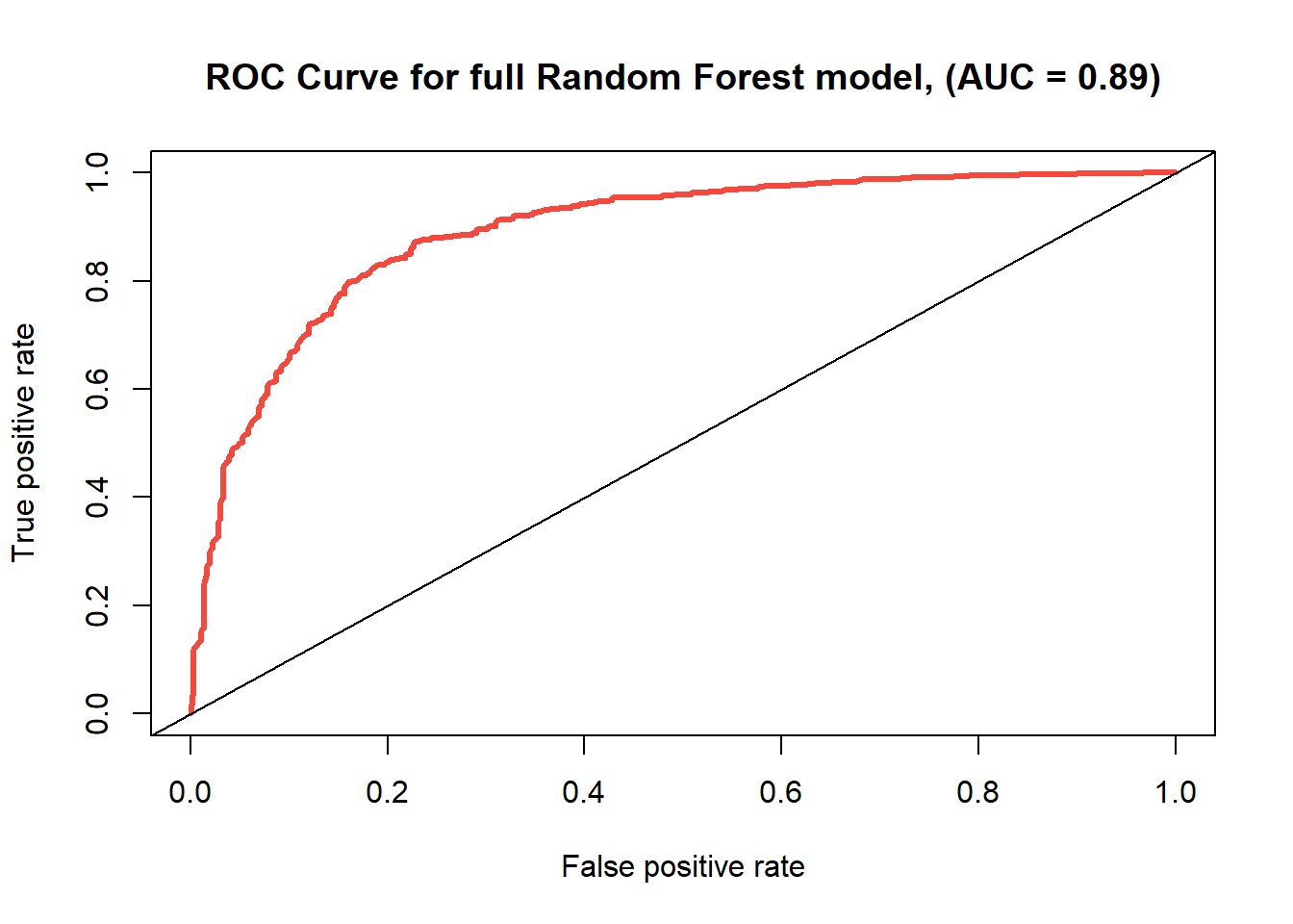
ROC Curve for full random forest with 8 variables.
| Accuracy Rate | Error Rate | AUC | |
|---|---|---|---|
| Repeated Cross-Validated Decision Tree | 0.739 | 0.261 | 0.746 |
| k=10 k-Nearest Neighbors | 0.756 | 0.244 | 0.689 |
| k=35 k-Nearest Neighbors | 0.755 | 0.245 | 0.741 |
| full Random Forest | 0.829 | 0.171 | 0.890 |
| small Random Forest | NA | NA | NA |
With an accuracy rate of 0.829, this random forest model is looking pretty good so far, and it already is more accurate than any method we’ve tried thus far. The area under the ROC curve for random forest is 0.892, which is also a strong AUC for a classification model and far above the competing models.
So we see actually that random forest stands head and shoulders above the other two methods, decision tree and k-nearest neighbors. This is seen in the fact that the accuracy rate, as well as the AUC, are the highest. Judging from this, we can assume that random forest would be the most likely to correctly classify a wine based off of the attributes and data given.
A smaller Random Forest model
We can look at a variable importance plot (See Figure @ref(fig:varImpPlot)) to see how the variables measure up against each other in terms of how relevant they are to the classification.
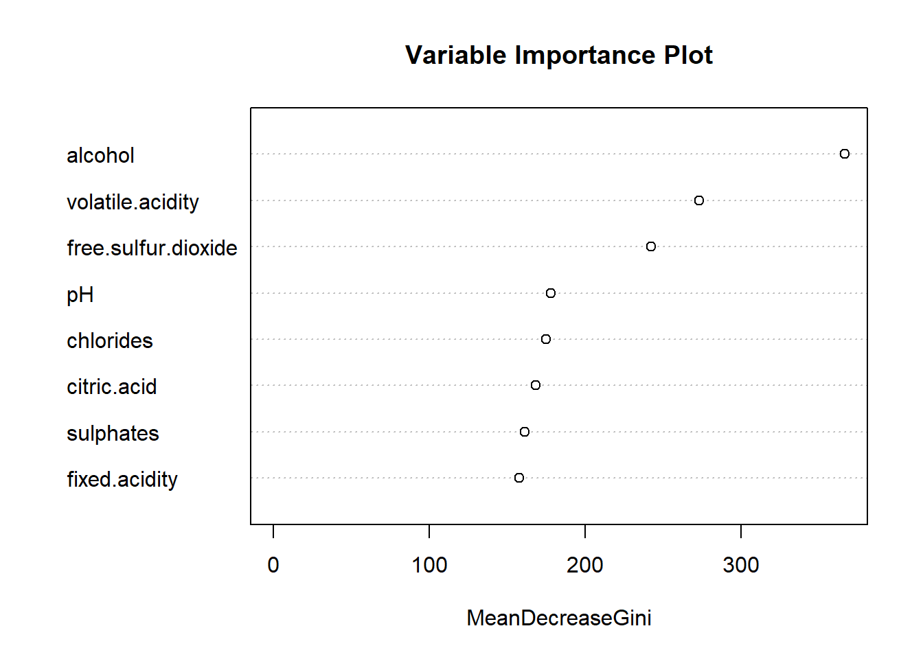
Variable Importance Plot comparing the Gini impurity index
meanDecreaseGini refers to the “mean decrease in node
impurity”. Impurity is a way that the optimal condition of a tree is
determined, and this plot shows how each variable individually affects
the weighted impurity of the tree itself.
This random forest model used all 8 of the predictor variables. This
variable importance plot shows how ‘important’ each variable was in
determining the classification. We can see that, consistent with the
decision tree, that alcohol, volatile.acidity,
and free.sulfur.dioxide are the three most important
predictors. While this random forest model was pretty effective in
utilizing all of the 8 predictors, we can take a look at a model using
only these 3 as well for the sake of comparison.
We have established by now that simpler models have a reduced bias and complexity, but higher variance and a higher chance of under-fitting, whereas complex models (such as the full model) have the opposite issue. The good thing about random forest is that it inherently accounts for this “Bias-Variance” trade-off by introducing randomness with bagging (bootstrap aggregating).
The question here is whether or not making the model simpler is worthwhile, but we can build the simple model and compare their metrics to find out. This comparison with the prior models can be seen in Table @ref(tab:records-5). The ROC curve for this model is depicted in Figure @ref(fig:partial-rf-roc) and the confusion matrix in Table @ref(tab:partial-rf-confmat).
set.seed(10)
rf2 <- randomForest(
  formula = quality ~ alcohol + volatile.acidity + free.sulfur.dioxide,
  data = train,
  mtry = 3
)
# predicting on the test set
rf_pred2 <- predict(rf2, test, type = "class")

# Confusion Matrix
rf_conf2 <- table(test$quality, rf_pred2)
rf_acc2 <- class_acc(rf_conf2)
rf_err2 <- 1 - rf_acc2

# Building the ROC Curve
rf_pred2 <- as.data.frame(predict(rf2, test, type = "prob"))
rf_pred_probs2 <- rf_pred2[, 2]
rf_roc_pred2 <- prediction(rf_pred_probs2, test$quality)
rf_perf2 <- performance(rf_roc_pred2,
  measure = "tpr",
  x.measure = "fpr"
)

# Area under the curve
rf_perf22 <- performance(rf_roc_pred2, measure = "auc")
rf_auc2 <- round(rf_perf22@y.values[[1]], 3)| bad | good | |
|---|---|---|
| bad | 228 | 130 |
| good | 72 | 570 |
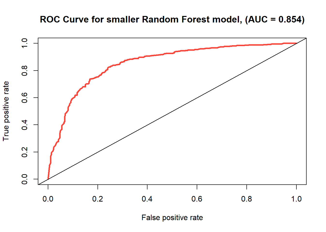
ROC curve for the random forest model using predictors ‘free sulfur dioxide’, ‘volatile acidity’, and ‘alcohol’.
| Accuracy Rate | Error Rate | AUC | |
|---|---|---|---|
| Repeated Cross-Validated Decision Tree | 0.739 | 0.261 | 0.746 |
| k=10 k-Nearest Neighbors | 0.756 | 0.244 | 0.689 |
| k=35 k-Nearest Neighbors | 0.755 | 0.245 | 0.741 |
| full Random Forest | 0.829 | 0.171 | 0.890 |
| small Random Forest | 0.798 | 0.202 | 0.854 |
The accuracy rate has actually decreased from 0.829 to 0.798, as well as the area under the curve from 0.892 to 0.854, but the model remains relatively strong, at least compared to the others. We’re managed to actually preserve the strength of the model, both in relation to the tree and k-nearest neighbor methods, but also relative to the original application of random forest with all of the predictors.
As such, we can opt to utilize this much smaller model for classification instead if we are concerned about complexity and bias. Having said that, because of the randomization introduced in the random forest, it is inherently more robust so sub-setting in this manner may not even be unnecessary.
Results
Now that we have accuracy and AUC metrics for all of the models, we can compare them on a plot to judge which is the best model. See Figure @ref(fig:final-comparison).
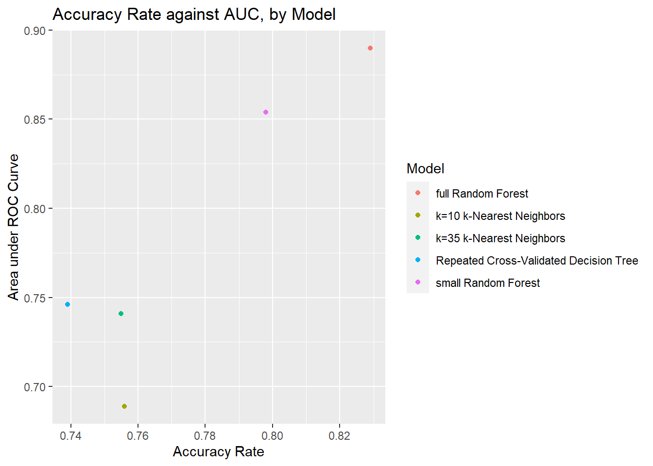
Scatterplot comparing AUC and Accuracy Rate of all models.
Looking at this plot of accuracy rate against AUC, it’s quite clear that the largest random forest model is the best one, even after downsizing the model to a subset of the predictors. With that said, the smaller random forest model still comes out much stronger than the competition in comparison.
Discussion
So judging from all of our findings, we have seen that in this case, random forest is the best algorithm (out of the three we’ve compared) for classifying this wine dataset. So we have answered the question of what among these three classification algorithms is truly the best.
The decision tree algorithm is useful but ultimately, random forest is superior version of it since it aggregates many decision trees to create an optimized model that is not susceptible to overfitting. When it comes to interpretability however, a decision tree is preferred. When using a decision tree however it is important to use cross-validation (ideally repeatedly) to ensure the tree does not overfit while retaining interpretability.
Compared to decision trees, the k-nearest neighbor algorithm has a
slightly greater accuracy rate but a worse AUC. The decision tree method
did however help to narrow down the three most relevant attributes:
alcohol, volatile.acidity, and
free.sulfur.dioxide. This finding was consistent with when
we took a look at the most important variables in the random forest
model.
We were able to apply this subset of attributes to the random forest algorithm and come out with a strong model that only utilizes a few independent variables in order to classify at a high success rate. This lends strength to the argument that these three variables are the most relevant when it comes to determining the content of a good wine.
As far as what these variables’ importance is in reality, is that sulfur dioxide is crucial for killing bacteria in wine when creating it. On the other hand, volatile acidity is an undesired trait in wine that affects flavor, that can be caused by such bacteria. So it makes sense that wine that is high in sulfur dioxide, and low in volatile acidity, is considered good.
The pending questions that remain are, did we overfit or underfit to
the training data when testing these different classification methods?
It is also worth determining exactly the threshold for the amounts of
these variables such as alcohol, for example finding the
optimal amount of alcohol content to create a good wine.
We would also like to delve more into how best to select some k for kNN that maintains a high level of accuracy while also having a balance between bias and variance without either over or underfitting. We would also posit a similar question for the number of nodes in a decision tree. Finally, is dropping variables in random forest really necessary, if the randomization inherent in it already accounts for overfitting?
If we can only compare models that utilize the same set of predictors, then we should look at the pruned classification tree against the random forest model utilizing the same attributes. We see even there that the random forest model is superior.
In conclusion we have found that random forest is best for binary classification and that alcohol, volatile acidity, and free sulfur dioxide are the most important predictors when attempting to classify a good wine.